
Regional Site Selection
Precipitation falling as snow on the surface of the Antarctic ice sheet is subject to reworking and transport downwind by katabatic and gradient wind systems. Thus snow accumulation at a site is a function of the regional precipitation rate, the wind regime, the snow density and the surface roughness. The latter largely controls the spatial variability of snow accumulation rates on the mesoscale (tens of km) to the microscale (tens of m). Therefore it is vital to have knowledge of the spatial variability across the regional surface of the ice sheet, to determine a representative site for ice core drilling.
The traditional method to measure the spatial variability of accumulation rates is to place marker canes at regular intervals across the ice sheet and measure the height of the snow surface at seasonal or annual intervals. More recently snow radar has been used by the Swedish Antarctic Research Programme (SWEDARP) and the US Antarctic Programme (USAP) to image the snow layers in the upper 10 metres of the snowpack to determine the spatial variability, and to verify the geographical representation of firn core sites in Dronning Maud Land, and West Antarctica, respectively.
Distinct snow layers are visible in the radar images (Figure 4). Each layer is interpreted as a buried surface and can be traced along the traversed profile. The radar signal is a function of snow density, and the depth-scale of the radar images is calculated from density data obtained from firn cores. The age of the snow layers can be determined by using stratigraphically dated firn cores as a control.
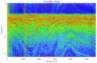
Figure 4 - An 800-2300 MHz radar profile of the surface snow layers along a section of the Swedish ITASE route in Dronning Maud Land (C. Richardson and P. Holmlund, Department of Physical Geography, Stockholm University, Sweden, pers. comm. 1996). The profile shows distinct layering in the upper 15 m of the snowpack which correspond to annual snow layers. Regions where folding occurs, particularly at the left of the profile, should be avoided for the retrieval of firn or ice cores, since the spatial variability would dominate the temporal signal. Sites with near horizontal laminar layering should be sought for firn and ice coring.
The folding in the firn and ice recorded by the radar, can reveal both unsuitable and suitable sites for ice coring (Figure 4). Regions where the snow layering is laminar over distances of a few kilometres offer the greatest potential for representative ice coring. It is important to avoid regions where there is considerable folding or interruption to the laminar snow layering, since the irregular snow structure was probably influenced by mesoscale topographic roughness. This roughness can have significant effects on the temporal variability of snow accumulation at a site since the snow at different depths has originated from different locations within the topography. For example, snow accumulating on a crest will be significantly less than that accumulating downwind in a trough or depression (Goodwin, 1990).
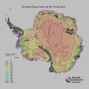
Figure 5 - Map of spatial accumulation across Antarctica, prepared by D. Vaughan et al., British Antarctic Survey, 1997, from an updated data compilation combined with the earlier compilation of Giovinetto and Bentley (1985).
The regional snow accumulation rate is also an important parameter to consider when selecting an ice core site. Figure 5 shows the spatial distribution of snow accumulation across Antarctica. Regions where snow accumulation is high relative to surface microrelief offer the greatest potential for obtaining detailed proxy climate records. Coastal regions are characterised by snow accumulation occurring during all seasons whereas in the interior snow accumulation is more sporadic, with the majority accumulating from winter snowfalls and hoarfrost. The snow accumulation rate also determines the depth of ice coring needed to retrieve a 200 year record, and hence, the type of drilling equipment required. Figure 6 shows the range of depths needed to penetrate 200 years in parts of West Antarctica.
Figure 6 - Map of West Antarctica showing the US ITASE traverse corridors together with the spatial distribution of snow depth to the 200 year isochron.
In order to understand controls on deposition for snow and impurities, it is necessary to follow trajectories of water- and impurity-laden air masses. After deposition, many of the ice sheet properties of interest are carried along by ice sheet flow. As a consequence, cross-sections or profiles that follow air flow trajectories or ice flow lines are valuable and necessary complements to any ground-based sampling. These studies allow physical and chemical changes and processes to be tracked all the way from atmospheric source regions, to deposition sites, then through the ice sheet to the ice core where the samples are recovered. Without these accompanying studies, interpretation of ground-based sampling would be difficult, processes controlling deposition would be unclear, and temporal gradients in deposition would be harder to separate from spatial gradients.
Core Analysis and Dating
Despite the importance of ice core research our current understanding of the spatial distribution of ice core properties over Antarctica is limited to a general knowledge of the surface distribution of ∂ 18O and a sparse surface sampling of selected major chemical species.
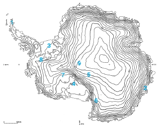
Figure 7 - The spatial distribution of mean annual surface values of ∂ 18O (Giovinetto et al., submitted) across Antarctica. The distribution is based on a multivariate analyses of measurements since 1982 and those in the compilation of Morgan (1982) on a 100 km grid.
The ∂ 18O of ice has classically provided the basic stratigraphy and paleoclimatology (temperature, moisture source) of ice cores. Giovinetto et al. (submitted) provides a survey of the Antarctic sites from which mean annual surface values of ∂ 18O have been recovered revealing the relative sparsity of measurements. The spatial distribution of mean annual surface values of ∂ 18O from Giovinetto et al. (submitted) is shown in Figure 7. Time series of ∂ 18O isotope measurements from a limited number of Antarctic ice cores covering the last ~1 kyr (Figure 8) reveal the regional complexity available from these records.
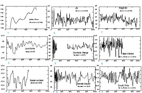
Figure 8 - Comparison of d18O series displaying Antarctic climate variability over the last ~1000 years. (M. Twickler, EOS, University of New Hampshire, pers. comm. 1997).
An understanding of the spatial distribution of the soluble and insoluble constituents in Antarctic snow and ice is essential to palaeoenvironmental and palaeoclimatic reconstructions. Based upon our present knowledge of the chemistry of the atmosphere, polar precipitation is expected to be composed of various soluble and insoluble impurities which are either introduced directly into the atmosphere as primary aerosols, such as seasalt (mainly sodium and chloride and some magnesium, calcium, sulfate and potassium) and continental dust (magnesium, calcium, carbonate, sulfate and aluminosilcates), or are produced within the atmosphere along various oxidation pathways involving numerous trace gases primarily derived from the sulfur, nitrogen, halogen and carbon cycles. In the case of the latter, the secondary aerosols and gases (H+, ammonium, chloride, nitrate, sulfate, fluoride, CH3SO3--, HCOO- and other organic compounds are derived from a variety of biogenic and anthropogenic emissions or volcanic activity. Measurements of soluble ionic constituents in snow and ice over Antarctica are valuable as indicators of changes in chemical species source strength and as tracers for atmospheric circulation yet relatively little information is available concerning their spatial variation over Antarctica (Figure 9). Further few measurements are available that cover overlapping time periods hence changes over time complicate spatial interpretations.
Figure 9 - Spatial distribution of snow chemistry data. a. All sites with surface snow glaciochemical measurements; b. Sites with surface snow chemical records longer than one year; c. Sites with surface snow chemical records from 1970-75; d. Sites with surface snow chemical records from 1980-85. (K. Kreutz, EOS, University of New Hampshire, pers. comm. 1997).
The first step in the ITASE ground-based sampling programme is to obtain a standardised suite of ice core properties (Table 1) which will be analysed on all ice cores collected within the ITASE programme. This will enable a cohesive spatial picture of Antarctic climate and environmental variability to be constructed. In addition to this standardised suite are a number of other properties which could be undertaken as opportunities for research within the ITASE programme (Table 2). Although it is expected that these measurements will be undertaken on a more limited scale than those listed in Table 1 these measurements provide significant additions to the understanding of climate and environmental change through, for example source fingerprinting (eg., trace metals and tephra).
Table 1 - Standardised ITASE ice core properties
Accumulation rate
Gamma-ray and beta detection
Electrical conductivity (ECM)
Physical properties (size, shape, arrangement of grains,
c-axis fabrics, depth-density analyses, melt layers,
visible strata)
Stable isotopes (δD, δ 18 O and deuterium excess)
Major chemistry (Ca, Mg, Na, NH4, K, Cl, SO4, NO3)
Microparticles    *
Other chemistry (F, I, Br, MSA, H2O2, HCHO)
Temperature
Table 2 - Opportunities for research
Cosmogenic isotopes (10Be, 36Cl, 26Al)
Radionuclides
Tephra
Trace metals (Se, Pb, Hg, V, Mn)
Trace elements (Cs, Rb, Ba, Sr)
Isotopes (Nd, Sr, Pb)
Trace Gases (CO2, CH 4, N2O, CFC's, CO, methyl-halides)
Biological particles (pollen, diatoms)
Biogenic compounds (DMSO, DMSO2)
Organic acids
Climate Variability Studies
Accumulation and Precipitation
Net snow accumulation at a site principally represents the original precipitation, together with some snow lost and/or gained due to surface wind redistribution, evaporation and sublimation. Snow accumulation rate time-series should be determined by at least two methods since this parameter is fundamental to the ITASE objectives as a proxy for precipitation. The existing data bank on accumulation has mostly been collected by repeated measurements on marker canes placed on the surface of the ice sheet, over periods of one year to a decade. Times series are required to determine a contemporaneous spatial distribution which can be used as a ground truth data set for comparisons with numerical analyses of the spatial precipitation pattern, derived from atmospheric moisture budgets (Cullather et al., 1996).
Since a variety of physical and chemical properties display an annual signal, they can be used to calculate the annual snow accumulation rate in a snow pit or on an ice core. These properties include:
- visible stratigraphic layering
- snow density cycles
- stable isotopes
- acidity measured as electrical conductivity (ECM)
- ionic chemistry
- hydrogen peroxide
The annual accumulation rate can also be determined using snow radar as discussed in section 3.1. This method produces a spatially continuous estimate of accumulation rate, together with interannual variability.
Estimates of the average accumulation rate can be made using Downhole Gamma Detector and Gross Beta Filtration methods. Downhole gamma ray detection will be used in every borehole to detect the depths to the atmospheric bomb test layers (1954-1965). Measurements of gross beta from Caesium 137 and other bomb products on cation filters from the recovered shallow cores also provide a tried-and-true determination of average accumulation rates over the past decades. The difference between the techniques is that the downhole gamma counter has the advantage that no dedicated core needs to be carried by the traverse vehicles while the beta filtration method requires less time at the core site.
Temperature and Humidity
Temperature
Temperature histories determined by the stable isotope temperature proxies should be calibrated at several sites by borehole temperature measurements (Cuffey et al., 1995; Clow et al., 1996), because stable isotopes can also reflect other changing climate parameters in addition to temperature.
Borehole temperature profiles should be measured immediately after drilling in order to detect modern spatial patterns of mean annual air temperature. It is unlikely that old 10-meter firn temperature data from the IGY era will be adequate to compare with modern data to detect recent temperature trends because there are too many sources of error associated with residual seasonal cycle effects at 10 meters, interannual variability, calibration offsets and air convection in open holes. However, it should be possible to directly measure temperature trends over the past 200 years by high-resolution (1 mK) continuous temperature logging.
Humidity
Histories of the polar air mass humidity can be determined from the measurement of deuterium excess in conjunction with the measurement of ∂ 18O and d D stable isotopes. These studies should be integrated with results derived from borehole measurements and spatial surveys to minimise confounding influences.
Atmospheric Circulation and Storm Frequency
Antarctic accumulation time series display strong interdecadal variability. Studies such as Cullather et al. (1996), have shown that the precipitation and hence accumulation time-series are linked to large scale circulation changes, linked to the ENSO phenomena. Changes in atmospheric circulation patterns in coastal Antarctica have been linked to oscillations in mean sea level air pressure (MSLP) within the circum-polar trough (Morgan et a., 1991 and Allan and Haylock, 1993). Increased annual snow accumulation in Wilkes Land has been associated with a decrease in MSLP in the quasi stationary cyclone position at E 110deg., a reduction in sea ice extent and concentration, and a poleward migration of coastal cyclone tracks (Goodwin, 1995). The ∂ 18O isotope record at Law Dome (van Ommen and Morgan, 1997) displays an enrichment greater than can be attributed to a warming air temperature alone. The ∂ 18O isotope enrichment has instead been explained as an indicator of more frequent storm or blizzard events, since the air temperature is close to zero during these events even in winter. Determination of the isotopic and chemical concentrations of each storm snow layer can distinguish the seasonal frequency and indicate the source regions of the storm activity during each seasonal event.
The chemical composition of an individual air mass provides a fingerprint that documents the history of the source area over which the transporting air mass passed. Therefore, atmospheric circulation systems can be labelled by the identification of the source areas that contribute to their chemistry. In the simplest case marine versus continental air masses can be differentiated based on the identification of seasalts (eg., NaCl) versus continental dusts (eg., CaSO4), respectively, in the chemistry of these air masses. More complex atmospheric circulation patterns and the frequency of storms events can be differentiated through statistical examination of the suite of major ions (Ca, Mg, Na, K, NH4, Cl, NO3, SO4) that comprise >95% of the soluble chemistry in the atmosphere (Mayewski et al., 1993, 1994, 1997).